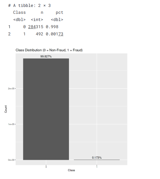
Credit card fraud is rare, and that's exactly what makes it hard to catch. In the dataset we worked with, only 492 out of 284,807 transactions were fraud, about 0.17%. A model can ignore fraud completely and still look almost perfect on paper.
This post walks through a data mining project I did with Richard Ung and Andrew Kiehn at San Jose State University, where we compared three models for detecting fraud: logistic regression, a decision tree, and a neural network. The full code is on Kaggle. Along the way, this post answers three questions:
- What is the business problem we're actually solving?
- Which metrics should we use to judge a model?
- Why does the choice of model matter?
Prefer to watch? I walk through the whole project in this video:
The business problem
A valid transaction is the real cardholder making a purchase. A fraudulent transaction is someone else using stolen card details.
The goal was to find a model that helps a fraud investigation team flag suspicious transactions in real time. Every new transaction gets scored as it happens. If it looks valid, it's approved right away. If it looks suspicious, it's flagged and sent to the fraud team. So a good model has to do two things at once: catch as much fraud as possible, and keep false alarms low enough that the team (and the customers whose cards get blocked) can live with them.
The data
We used the well-known credit card fraud dataset of European
cardholders' transactions. Instead of readable columns like
merchant, location, or category, most of its features are named
V1 to V28. They were produced with
principal component analysis (PCA), which transforms the original
data to protect cardholders' privacy. We can model these features,
but we can't interpret them. Only Time and
Amount are left in their original form.
We also checked a correlation heatmap of the features. Correlations were mostly low to moderate, so there was no small group of features that obviously drove fraud on its own. That hinted that a straight-line decision boundary might not be enough, and that more flexible models could have an advantage.
Splitting the data carefully
With fraud this rare, a plain random split can leave the test set with very few fraud cases, or in the worst case none. Then every number you compute afterwards is unreliable. We sampled 20% of the fraud rows and 20% of the valid rows separately, so both the training and test sets keep the same fraud rate. We did this in R:
idx1 <- which(df$Class == 1)
idx0 <- which(df$Class == 0)

test_frac <- 0.20
test_idx1 <- sample(idx1, size = floor(length(idx1) * test_frac))
test_idx0 <- sample(idx0, size = floor(length(idx0) * test_frac))
test_idx  <- c(test_idx1, test_idx0)
train_idx <- setdiff(seq_len(nrow(df)), test_idx)

train <- df[train_idx, , drop = FALSE]
test  <- df[test_idx, , drop = FALSE]
This gave a test set of 56,961 transactions, 98 of them fraud. All the results below come from that test set.
Choosing the right metrics
First, what not to use: accuracy. A model that approves every single transaction is right 99.83% of the time on our test set, and it never catches a single fraud.
Instead we start from the confusion matrix, which splits predictions into four groups:
| Model says fraud | Model says valid | |
|---|---|---|
| Actually fraud | True positive: fraud caught | False negative: fraud missed |
| Actually valid | False positive: false alarm | True negative: valid purchase approved |
From those counts we get three metrics:
- Precision: of everything we flagged, how much was really fraud? Low precision means blocked cards, annoyed customers, and more calls to support.
- Recall: of all the real fraud, how much did we catch? Low recall means fraud slips through and the bank pays for it.
- F1 score: one number that balances precision and recall (their harmonic mean). It's useful when both kinds of mistake matter.
The three models
Logistic regression
Logistic regression draws a straight-line boundary between fraud and valid transactions. Its big strength is transparency: each coefficient shows how a feature pushes the odds of fraud up or down, which is why it's so common in banking and credit risk, where models have to be explained to regulators.
We used backward stepwise selection: start with every feature, drop the least significant one, refit, and repeat. The final model kept 17 predictors. It works, but it means fitting the model many times in a row, which matters when we look at training time.
Decision tree
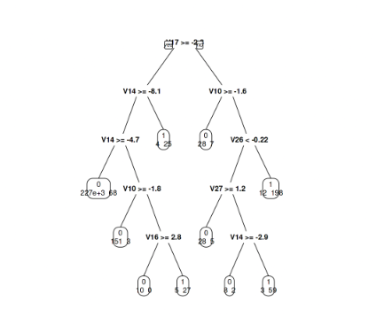
A decision tree splits the data with simple yes-or-no rules, like "if V14 is below −8.1, flag as fraud." You can print the whole model on one page and walk a non-technical stakeholder through it.
Neural network
The neural network has hidden layers with ReLU activations, dropout layers to reduce overfitting, and a softmax output that gives the probability of fraud. Unlike logistic regression, it can learn curved, complex boundaries between the classes, which is what the correlation heatmap suggested we might need.
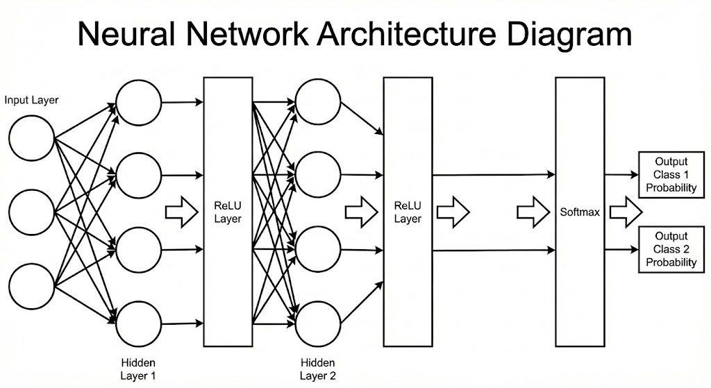
We chose ReLU because it avoids the saturation problem of sigmoid and tanh, where gradients shrink toward zero and earlier layers stop learning (the vanishing gradient problem). For the neural network, we flagged a transaction as fraud when its predicted probability was above 0.148, the cutoff that gave the best F1 score.
Results
| Model | Precision | Recall | F1 | AUC | Accuracy |
|---|---|---|---|---|---|
| Logistic regression | 0.742 | 0.735 | 0.739 | 0.979 | 0.9991 |
| Decision tree | 0.895 | 0.786 | 0.837 | 0.893 | 0.9995 |
| Neural network | 0.863 | 0.837 | 0.850 | 0.943 | 0.9995 |
A few things stand out:
- Accuracy is useless here. All three models score above 99.9%, and so does doing nothing.
- The tree has the best precision, the neural network has the best recall, and their F1 scores are almost tied (0.837 vs 0.850).
- Logistic regression trails on precision, recall, and F1, even though it has the highest AUC. More on that below.
Since precision and recall are just ratios, it helps to look at the actual counts behind them:
| Model | Frauds caught | Frauds missed | False alarms |
|---|---|---|---|
| Logistic regression | 72 / 98 | 26 | 25 |
| Decision tree | 77 / 98 | 21 | 9 |
| Neural network | 82 / 98 | 16 | 13 |
Why the highest AUC didn't win
Logistic regression had the best AUC (0.979) but the worst F1. That sounds contradictory, but they measure different things. AUC looks at how well a model ranks transactions from most to least suspicious, across every possible cutoff. Precision, recall, and F1 are measured at the one cutoff you actually use to flag transactions.
So logistic regression was good at sorting transactions by risk, but at the cutoff it used it didn't separate fraud from valid transactions as well as the other two models. A different cutoff might narrow the gap, which is something I'd test next time.
Training time
| Model | Training time (CPU only) |
|---|---|
| Decision tree | 68.8 s |
| Neural network | 132.9 s |
| Logistic regression | 1,053.4 s |
Logistic regression took about 15 times as long as the tree. That's not because logistic regression is slow (a single fit is usually the fastest of the three). It's because backward stepwise selection refits the model again and again as it drops features. The neural network took about twice as long as the tree, which is a reasonable price for its extra recall.
Why we chose the neural network
The neural network and the decision tree finished with nearly the same F1, but they get there in different ways. The tree is picky: when it flags something, it's usually right, but it lets more fraud through. The neural network catches more fraud while keeping false alarms low, and in fraud detection a missed fraud is a direct financial loss while a false alarm is a cheap review.
The other two models still have a place. Logistic regression is the easiest to explain to regulators, and the tree's rules are easy for a fraud team to read and act on. If interpretability were a hard requirement, either would be a reasonable choice. But for catching the most fraud, the neural network is the best fit.
Bonus: does it hold on a different dataset?
To check that we hadn't just tuned our way into one dataset's quirks, we trained the same three models on the German Credit dataset, where the task is to predict which loan applicants are a bad credit risk.
| Model | Precision | Recall | F1 | AUC | Accuracy |
|---|---|---|---|---|---|
| Logistic regression | 0.730 | 0.258 | 0.381 | 0.722 | 0.807 |
| Decision tree | 0.705 | 0.332 | 0.452 | 0.722 | 0.814 |
| Neural network | 0.935 | 0.735 | 0.823 | 0.740 | 0.774 |
The neural network came out on top again, with the best precision, recall, F1, and AUC. The other two models caught only about a quarter to a third of the positive cases.
Notice the accuracy column, though. The neural network has the lowest accuracy of the three, while the decision tree has the highest. If we had ranked models by accuracy, we would have picked the model that misses two-thirds of the cases we care about. It's the same lesson as the fraud data, from a different angle.
Takeaways
- Split imbalanced data by class. Sample the rare class and the common class separately, so every split contains enough positive examples to learn from and to evaluate on.
- Don't judge models by accuracy when one class is rare. Look at the confusion matrix, precision, and recall.
- Look past a tied F1. When two models score the same, ask which kind of mistake hurts the business more, and pick the model that makes fewer of those.
- AUC and F1 answer different questions. A model can rank risk well and still perform poorly at the cutoff you actually use.
- Interpretability is a real trade-off. The best model on the metrics isn't always the one you can deploy, so know what your stakeholders and regulators need before you choose.
This project was completed in December 2025 for a data mining course at San Jose State University, taught by Professor Shaonan Tian, with teammates Richard Ung and Andrew Kiehn. Models were built in R.
Source: Data Mining using NN for Credit Fraud Detection (Kaggle notebook)