This fall I competed solo in the RSNA 2026 Knee Abnormality Detection competition on Kaggle. My best entry scored 0.958 on the public leaderboard. When the private leaderboard was revealed, it scored 0.942 and finished 1,740th out of 6,425 teams, in the top 27%.
The more interesting number: 1,322 teams finished with exactly 0.942. Almost everyone who built on the same popular public notebooks ended up in one giant tie. This post is about how that happened, what I built along the way, and what the teams at the top did differently.
The competition in plain terms
The task was to look at a full knee MRI study (several series of images taken from different angles, each with dozens of slices) and predict the probability of 12 findings: ACL and MCL tears, medial and lateral meniscus tears, osteoarthritis in three parts of the knee, joint effusion, synovitis, Baker's cyst, bone contusion, and fracture. There were about 4,400 studies to train on.
A few rules shaped everything:
- Scoring was macro AUC: the AUC of each finding, averaged across all 12. AUC measures how well a model ranks positive cases above negative ones, so a rare finding counts as much as a common one.
- It was a code competition. You submit a notebook, and Kaggle runs it on hidden test studies with a 9-hour GPU limit. You get 5 submissions a day and pick 2 for the final ranking.
- The labels came from radiology reports, not from experts looking at the images. Only 58 "gold" studies had labels from expert radiologists reading the images directly.
That last point turned out to be the whole competition. A report tells you what a radiologist chose to mention, not everything that is on the images. Small findings go unmentioned, different hospitals write reports differently, and "small effusion" may or may not count as positive by the experts' definition. So the training labels were noisy, and the only trustworthy validation set had 58 studies in it.
What I built
Phase 1: my first models
I started with standard image models: ConvNeXt-Tiny and EfficientNetV2-S, each reading stacks of MRI slices and predicting all 12 findings at once. For labels, I combined several public tables of findings extracted from the reports, then mixed in the out-of-fold predictions of one image model. Measured against the 58 gold studies, that raised label quality from 0.896 to about 0.92 AUC, which helped more than any change to the models themselves.
On their own, these first models scored 0.941 on the public leaderboard.
Phase 2: climbing the public leaderboard
Several strong public notebooks were shared during the competition, especially the Raptor models and heliosli's R6, R7, and S6 models. Blending them with my own models climbed the public leaderboard quickly:
| Entry | Public | Private |
|---|---|---|
| One of my EfficientNetV2-S models alone | 0.937 | 0.923 |
| Raptor + my models | 0.950 | 0.935 |
| Raptor + heliosli S6, plus my models at 15% | 0.954 | 0.937 |
| Raptor + heliosli R7, plus my models at 15% | 0.956 | 0.940 |
| heliosli's blend notebook, unchanged | 0.958 | 0.942 |
Two lessons came out of this phase. First, diversity beats strength in a blend: adding a model that makes different mistakes helps more than adding a slightly better model that makes the same ones. Second, my own models mattered less and less. By the end, the best public blends used outside models at only 1–3% weight, and my top-scoring entry was a public notebook with nothing of mine in it.
Phase 3: a better model of my own (v2)
I didn't want to finish with only other people's work, so I built a second-generation model from scratch. It's a ConvNeXt-Small with a few ideas about how the images are fed in:
- Every knee faces the same way. Left knees are mirrored so the model always sees the same anatomy in the same place.
- Two views per series: the full 160 mm field of view, plus a 110 mm close-up centred on the joint. The centre comes from a knee segmentation model rather than the middle of the image.
- It reads every slice (up to 48 per series) and keeps each slice's position in millimetres, instead of sampling a fixed handful.
I trained it on three folds on Google Colab with an A100 GPU, about 4.5 hours per fold. On its own it scored 0.943 public. Here's how it compares with the other models on the 58 gold studies, finding by finding:
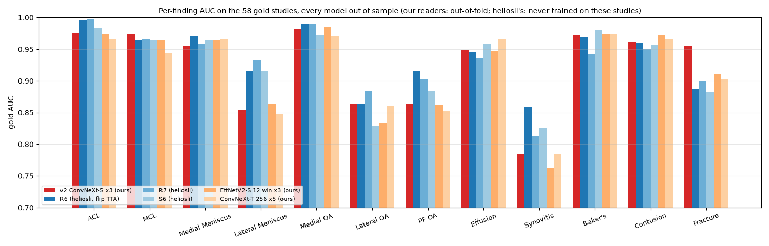
v2 was the best model I tested on fracture (0.956 vs 0.888 for the strongest public model) and slightly better on MCL. It was clearly weaker on synovitis, lateral meniscus, and patellofemoral osteoarthritis. Its average across all 12 findings (0.924) was below the best public model (0.937). Adding it to the public blends never raised the public score.
Phase 4: the engineering pain
A surprising amount of time went into notebooks that worked perfectly on my machine and broke only on Kaggle. The Kaggle image ran Python 3.13, which my DICOM image decoders didn't support out of the box. The T4 GPUs don't handle bf16 the way the A100 I trained on does. And one submission failed only on the hidden test set, which I never get to see. The fix was defensive inference: processing the model in chunks, retrying on out-of-memory errors, and tolerating a few images that fail to decode instead of crashing the whole run.
The shake-up
The public leaderboard is scored on a small part of the test set. The private leaderboard, revealed at the end, uses the rest. Here is how my main entries moved:
| Entry | Public | Private | Drop |
|---|---|---|---|
| Best public-notebook blend | 0.958 | 0.942 | 0.016 |
| Public blend + my first models | 0.946 | 0.931 | 0.015 |
| My v2 model alone | 0.943 | 0.928 | 0.015 |
| My first models alone | 0.941 | 0.928 | 0.013 |
Every entry dropped by a similar amount, and the order barely changed. The problem wasn't overfitting to the public board in the usual sense. It was that blends of the same public models had a ceiling: on the private leaderboard they all landed between 0.942 and 0.944, no matter how they were weighted. Over a thousand teams hit that ceiling, which is where the 1,322-way tie comes from. The top teams also dropped from public to private, but only by 0.009 to 0.013, and the winners finished at 0.960.
What the top teams did differently
After the competition, many of the top teams published write-ups (for example 5th, 7th, and 8th place), and TaeyanG4 collected them in a helpful index. Reading through them, three things kept coming up.
1. They fixed the labels by looking at the images
This was the biggest difference. Top teams had vision-language models (AI models that can read images and text) look at the actual MRI slices, often one study at a time with the experts' grading rules, and combined those image readings with the report labels finding by finding. Their labels agreed with the expert gold labels at around 0.947–0.952 AUC. Mine reached about 0.92. A model can only learn what its labels teach it, so that gap carried straight through to the final scores.
2. They removed a hidden shortcut: the hospital
The studies came from many hospitals, and each one writes reports differently. Some mention small findings far more often than others. Scanner settings reveal which hospital a study came from almost perfectly, so a model can learn "this hospital reports lots of effusion" instead of "this image shows effusion." Several top teams added a hospital correction term that's used during training and dropped at test time. It was worth +0.006 to +0.014 on its own.
3. They matched the labels to the experts' definitions
A finding that isn't mentioned in a report isn't the same as a confirmed negative, and a "small" effusion may not meet the experts' threshold for positive. Teams that re-mapped report wording to the experts' definitions saw their label quality jump, in one case from 0.902 to 0.947 against the gold set.
The good news
The way my v2 model reads the images (same orientation for every knee, anatomy-centred close-ups, every slice, positions in millimetres) was very close to what the medal teams used. The 7th-place team's best single model used nearly the same setup. The gap between my v2 at 0.928 private and their single models at around 0.958 was mostly the labels it was trained on, not the architecture.
Lessons learned
- Labels are the biggest lever. In my own work, improving the labels did more than any model change, and the top teams proved it at a larger scale. When the labels are noisy, fix them before tuning the model.
- The public leaderboard can be a trap. When everyone is blending the same public models, a higher public score mostly tells you that you're closer to everyone else. Ask what your work adds that the public notebooks don't.
- A tiny validation set can't rank models. 58 studies is too few to choose between models that differ by a fraction of a point. When I tuned per-finding weights on the gold set, the public score went down, and the top teams reported the same.
- Look for shortcuts in the data. If something like the hospital or scanner predicts the label, the model will happily learn it instead of the medicine.
- Test in the real environment early. Most of my failures happened only on Kaggle's machines, and the worst one only on the hidden test set.
If I did it again
- Spend the first weeks on labels: have an image-reading model look at every study, combine its readings with the reports, and map everything to the experts' definitions.
- Add a training-only hospital correction, and keep studies from the same hospital in the same validation fold.
- Keep the v2 input design, which already matched the winners.
- Stop tuning blends of public notebooks early, since their ceiling was clear well before the deadline.
My v2 model and its full write-up, including how it was built and trained, are on Kaggle: RSNA Knee v2 single model.
Thanks to heliosli and the author of Raptor for sharing their notebooks publicly, and to the top teams for publishing such detailed write-ups. Scores for other teams are from their own write-ups.